Ontario Cancer Statistics 2022 Analysis
What's on this page
Significance Testing
Throughout this report, the word “significant” refers to statistical significance at an alpha level of 0.05 for changes in trend or when comparing differences in rates or ratios. When referring to changes in trends, statistically non-significant changes are described in this report as "stable." Any other noted trend changes (increasing or decreasing) are statistically significant. In some instances (such as for survival statistics), statistical significance is assessed using a confidence interval, which accounts for variations and chance errors and represents the frequency with which the interval would contain the average measure 19 times out of 20 (or 95% of the time).
Probability of Developing or Dying From Cancer
The probability of developing or dying from cancer refers to the probability of a newborn child developing or dying from cancer at some point during their lifetime. Lifetime risk calculations are based on current incidence and mortality rates. Therefore, these risk calculations assume that the current rates within each age group will remain constant during the life of the newborn child.
The probability of developing or dying from cancer was calculated using DevCan software.(1) The DevCan software program uses life-table methods based on cross-sectional incidence, mortality and population data for 18 age groups to compute the lifetime and age-conditional probabilities of developing or dying from cancer.
Projections
Incidence and mortality
Projections of incidence and mortality for 2019 to 2022 were estimated using the Canproj projection package(2) in R software.(3) The Canproj package is a modified version of Nordpred Power 5 package,(4) which is based on an age-period-cohort Poisson regression model. The Canproj package has enhancements that overcome difficulties in the standard Poisson model and improve projection accuracy.
The Ontario populations used for the cancer projections were from population projections up to 2046 derived by the Ontario Ministry of Finance. The methodology and assumptions for the projected populations can be found elsewhere.(5)
Canproj consists of 3 sub-packages:
- Nordpred model (adpcproj: age-drift-period-cohort model)
- age-cohort model (acproj: age-cohort model)
- hybrid model (hybdproj: age-only model)
Each sub-package can work independently for projections. Canproj has a built-in decision tree to help determine which of the 3 models is most appropriate. The package can also replace the Poisson distribution to a negative-binomial distribution when overdispersion is present in the data. Finally, Canproj tests the goodness-of-fit of the chosen model.
Projections for "all cancers" and each individual cancer site were estimated using the Canproj package.
Age-drift-period-cohort model (Nordpred)
The Norpred Power 5 model is represented as:
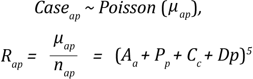
where the symbols represent the following:
- Rap is the incidence rate in age group a in calendar period p.
- μap is the mean count of cases in age group a in calendar period p.
- nap case is the size of the corresponding population.
- Aa is the age component for age group a.
- D is the common linear drift parameter.
- Pp is the non-linear period component of period p.
- Cc is the non-linear cohort component of cohort c.
- p is the calendar period,
Cohorts were calculated as c = A + p - a with A equaling the total number of age groups.(2)
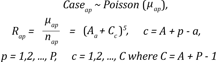
Age-cohort model (acproj model)
The age-cohort model is a reduced form of the Nordpred model selected by Canproj when sparse data exist in the youngest and oldest birth cohorts. Due to sparseness of the data at both extreme cohorts, the remaining cohorts with complete observations are set as reference when age and cohort affects are being estimated.(2)
The expression for the age-cohort model is
Hybrid models: age-only, common trend and age-specific trend models
There are 3 types of hybrid models: age-only, common trend and age-specific. The models use a combination of 3 methods: average, joinpoint type and whenever the cohort effects are not significant, Poisson regression methods.(2,6) The hybrid functions first compare the common trend model with the age-specific model using a chi-square test in the age groups where data exist for the entire periods. When there is no significant difference between the models, the common trend is preferred; otherwise, age-specific is preferred.
The incidence, death and population data were classified by year of diagnosis, year of death and sex, and grouped by 5-year age groups (0 to 4, 5 to 9 … 85 and older). For incidence projections, cases meeting the International Association for Research on Cancer/International Association of Cancer Registries multiple primary rules from 1984 to 2018 were projected. These were later converted for the 2010 to 2016 period for Surveillance, Epidemiology and End Results multiple primary rules by applying an inflation factor based on the age-specific increase in multiple primary cancers. Projections for all cancers combined were estimated based on the sum of all data from the 23 cancer sites in this report.
Mortality projections were also made with a Canproj package using cancer deaths from 1984 to 2018 divided into 5-year age groups and calendar year. To get incidence and mortality projections for all cancers combined, projections were calculated by sex and then summed. This method was used because the projections based only on the data for all cancers combined are not equal to the sum of the projections for males and for females. The lists of models used for all cancers combined and for each individual cancer site by sex are in Table A.6 for incidence projections and Table A.7 for mortality projections.
| Cancer type | Sex | |
|---|---|---|
| Males | Females | |
| All cancers | adpcproj (NB) | adpcproj (NB) |
| Bladder | adpcproj (NB) | adpcproj (P) |
| Brain | acproj (P) | adpcproj (P) |
| Breast (female) | n/a | adpcproj (NB) |
| Cervix | n/a | adpcproj (P) |
| Colorectal | adpcproj (NB) | adpcproj (NB) |
| Esophagus | hybdproj (Avg) | hybdproj (ComT) |
| Hodgkin lymphoma | hybdproj (NBags) | acproj (P) |
| Kidney | adpcproj (NB) | hybdproj (NBags) |
| Larynx | adpcproj (P) | adpcproj (P) |
| Leukemia | hybdproj (NBags) | hybdproj (NBags) |
| Liver | adpcproj (NB) | adpcproj (NB) |
| Lung | adpcproj (NB) | adpcproj (NB) |
| Melanoma | adpcproj (NB) | adpcproj (NB) |
| Myeloma | adpcproj (P) | hybdproj (ComT) |
| Non-Hodgkin lymphoma | adpcproj (P) | adpcproj (P) |
| Oral cavity and pharynx | adpcproj (P) | adpcproj (P) |
| Ovary | n/a | adpcproj (NB) |
| Pancreas | hybdproj (NBags) | hybdproj (ComT) |
| Prostate | adpcproj (NB)† | n/a |
| Stomach | adpcproj (P) | adpcproj (NB) |
| Testis | hybdproj (ComT) | n/a |
| Thyroid | adpcproj (P) | adpcproj (NB) |
| Uterus | n/a | adpcproj (P) |
Abbreviations:
- acproj (P) means age-cohort model with Poisson distribution
- acproj (NB) means age-cohort model with negative-binomial distribution
- adpcproj (NB) means Norpred model with negative-binomial distribution
- adpcproj (P) means Norpred model with Poisson distribution
- hybdproj (NBags) means hybrid model with age-specific and negative-binomial distribution
- hybdproj (Ags) means hybrid model with age-specific and Poisson distribution
- hybdproj (ComT) means hybrid model with common-trend
- hybdproj (Avg) means hybrid model with average method
- n/a means “not applicable”
Symbol: † Five periods were used to estimate projected incidence. Projected estimates used data starting from the 35- to 39-year age group.
| Cancer type | Sex | |
|---|---|---|
| Males | Females | |
| All cancers | adpcproj (P) | adpcproj (NB) |
| Bladder | adpcproj (P) | hybdproj (ComT) |
| Brain | adpcproj (P) | adpcproj (NB) |
| Breast (female) | n/a | adpcproj (NB) |
| Cervix | n/a | adpcproj (P) |
| Colorectal | adpcproj (P) | adpcproj (P) |
| Esophagus | hybdproj (NBags) | hybdproj (ComT) |
| Hodgkin lymphoma | hybdproj (Ags) | hybdproj (ComT) |
| Kidney | acproj (P) | adpcproj (P) |
| Larynx | hybdproj (Ags) | adpcproj (P) |
| Leukemia | adpcproj (P) | hybdproj (Ags) |
| Liver | adpcproj (P) | adpcproj (P) |
| Lung | adpcproj (NB) | adpcproj (P) |
| Melanoma | acproj (P) | acproj (P) |
| Myeloma | hybdproj (NBags) | acproj (NB) |
| Non-Hodgkin lymphoma | adpcproj (P) | adpcproj (P) |
| Oral cavity and pharynx | hybdproj (NBags) | hybdproj (NBags) |
| Ovary | n/a | adpcproj (P) |
| Pancreas | hybdproj (Avg) | acproj (NB) |
| Prostate | adpcproj (NB)† | n/a |
| Stomach | adpcproj (P) | adpcproj (NB) |
| Testis | hybdproj (ComT) | n/a |
| Thyroid | hybdproj (ComT) | hybdproj (Avg) |
| Uterus | n/a | adpcproj (P) |
Abbreviations:
- acproj(P) means age-cohort model with Poisson distribution
- acproj(NB) means age-cohort model with negative-binomial distribution
- adpcproj (NB) means Norpred model with negative-binomial distribution
- adpcproj (P) means Norpred model with Poisson distribution
- hybdproj(NBags) means hybrid model with age-specific and negative-binomial distribution
- hybdproj(Ags) means hybrid model with age-specific and Poisson distribution
- hybdproj(ComT) means hybrid model with common-trend
- hybdproj(Avg) means hybrid model with average method
- n/a means “not applicable”
Symbol: † Six periods were used to estimate projected incidence. Projected estimates used data starting from the 45- to 49-year age group.
Prevalence
Prevalence projections can be interpreted as the effect of the growth and aging of the Ontario population and current cancer control strategies. Projections for 2019 to 2034 were estimated using the Prevalence and Incidence Analysis Model (PIAMOD), which is a unified statistical package for estimating and projecting complete prevalence of cancer.(7)
Prevalence projection in PIAMOD requires several types of input data, such as cancer incidence, population and all-cause mortality. To this end, annual observed incidence data by cancer type (from 1984 to 2018) were extracted from the Ontario Cancer Registry and were restricted to first primaries. Ontario population and all-cause mortality were obtained from Statistics Canada databases for single years of age (0, 1, 2 … 90+ years old).
Age-cohort models with different parameters were fitted to the historical cancer- and sex-specific incidence data in the PIAMOD software. The best age-cohort models were selected based on the lowest likelihood ratio test statistic and fewest parameters. The selected cancer- and sex-specific age-cohort models are shown in Table A.8. The estimated parameters from the selected age-cohort models and tabulated relative survival rates estimated from SEER*Stat software(8) were used for annual age-specific prevalence projections by sex and cancer type (including all cancers combined) in PIAMOD. The projected counts are used to calculate prevalence proportion and standardized to 2011 Canadian Standard population. A validation of the PIAMOD projected prevalence estimates was conducted by comparing the actual prevalence obtained through the direct counting method or limited-duration prevalence estimation with the PIAMOD projected estimates for the year 2018. The relative percentage differences between the limited-duration and PIAMOD prevalence estimates were generally between 0.34% and 13%, in both males and females.
| Cancer site | Males | LRS | Females | LRS |
|---|---|---|---|---|
| All cancers | AC701 | 8285.9 | AC603 | 4705.1 |
| Breast (female) | n/a | n/a | AC603 | 3942.4 |
| Colorectal | AC205 | 3147.3 | AC505 | 2708 |
| Kidney | AC404 | 2519.7 | AC401 | 2406.7 |
| Leukemia | AC602 | 3234 | AC303 | 2967.6 |
| Lung | AC404 | 2707.2 | AC404 | 2667.2 |
| Melanoma | AC205 | 2977.6 | AC402 | 3000.6 |
| Non-Hodgkin lymphoma | AC404 | 3014.9 | AC403 | 2807.6 |
| Prostate | AC503 | 20689.4 | n/a | n/a |
| Thyroid | AC203 | 2237.4 | AC404 | 3893.8 |
| Uterus | n/a | n/a | AC402 | 2627.7 |
Abbreviations: AC means age-cohort model; LRS means likelihood ratio statistic; n/a means not applicable.
Incidence and Mortality
Counts
Incidence counts are the number of new cancer cases diagnosed in a population during a specific period. ln this report, incidence counts refer to the number of new cancer diagnoses in a calendar year in Ontario. At the time of writing, complete death-cleared incidence data were available up to 2018.
Mortality counts describe the number of deaths attributed to cancer during a specific period in a specific population. ln this report, mortality refers to the number of deaths due to cancer in a calendar year in Ontario. For consistency, this report uses data for the same range of years for incidence and mortality (i.e., 1984 to 2018).
The childhood cancer incidence statistics included this report are based on the cohort of children diagnosed with cancer from 1986 to 2020 and are presented for 1986 to 2020. Childhood cancer mortality statistics are based on the cohort of children diagnosed with cancer from 1986 to 2019 and are presented for 1991 to 2019.
Rates
Incidence and mortality rates are the number of new cancer cases or deaths per 100,000 people in a population during a specific period. Rates presented by sex are per 100,000 males or per 100,000 females in the population during the specified period. The rates are sometimes called crude rates because they do not adjust for the age distribution of the population. Rates were calculated using SEER*Stat v.8.3.8.(8)
For children with cancer (ages 0 to 14), incidence and mortality rates are the number of new cancer cases or deaths per 1,000,000 people in the population during a specific period. Childhood cancer rates were calculated using Statistical Analysis System v.9.4.(9)
Age-standardized rates
Age-standardized rates are weighted averages of age-specific rates using a standard population. Age-standardized incidence rates and age-standardized mortality rates are adjusted for differences in the age structure of different populations. This adjustment permits comparisons of cancer incidence or mortality between different populations, which may be different segments of a population (e.g., different geography) or the same population at different times. An age-standardized rate gives the rate that would have occurred if the population had the same age distribution as the standard population.
This report uses direct standardization, which produces artificial rates for the purpose of comparison only. The standard population used is based on the 2011 Canadian Standard population (with 5-year age groups).
Trends in age-standardized rates
Incidence and mortality trends were determined using annual percent change and average annual percent change, and calculated using age-standardized rates. Annual percent change was used when examining short-term changes in trend. Average annual percent change is a summary measure that describes the change in trend over a longer period with a single statistic.
Annual percent change and average annual percent change statistics were produced using the Joinpoint Regression Program (version 4.8.0.1).(10,11) The Joinpoint software uses piecewise regression to model the change in rates on the log scale.
The Joinpoint software uses a statistical algorithm to interpret data and determine statistically significant changes in trend. The software chooses the best points for a trend to change (called joinpoints) and how many changes there should be. Joinpoint uses the Monte Carlo Permutation test to determine whether the change in trend is statistically significant.(4) ln general, the model that the Joinpoint software found to be the best fit was used. A maximum of 3 joinpoints and a minimum of 5 data points between joinpoints were allowed.
Jump model for incidence trend analysis
For most cancer sites, the standard joinpoint model (see above) was used to analyze incidence trends. Furthermore, these analyses only included cancer cases meeting the International Association for Research on Cancer/International Association of Cancer Registries criteria for multiple primary cancers.
However, for selected cancer sites, the jump model was used instead of the standard joinpoint model to analyze trends in age-standardized incidence. The jump model is an option available in the Joinpoint software to estimate trends in situations where a coding change has resulted in a sudden shift (or “jump”) in cancer rates. Since a shift in rates caused by a coding change is assumed to be artificial, the jump model accounts for this type of shift to produce estimates of the underlying trend.(12)
In this report, the jump model was used for the following cancer sites for cases meeting the National Cancer lnstitute’s Surveillance, Epidemiology and End Results Program’s criteria for multiple primaries (see Coding Rules for Multiple Primary Cancers):
- all cancers
- bladder
- breast (female)
- melanoma
For all cancers, melanoma and breast (female), an abrupt increase in incidence rates was observed due to the impact of applying the Surveillance, Epidemiology and End Results rules for cases diagnosed from 2010 onwards. For bladder cancer, an abrupt increase in incidence rates occurred primarily due to the inclusion of in situ bladder cases, also from 2010 onwards. The jump model accounted for these artificial increases to produce estimates of the underlying trend.
Survival
In this report, survival analyses measure net cancer survival. Net survival is the probability of surviving cancer in the absence of other causes of death. It is a measure that is not influenced by changes in mortality from other causes and is therefore a useful way to track cancer survival across time, as well as between population groups and between registries. The measure of net survival used in this report is the relative survival ratio. Relative survival ratios are estimated by comparing the survival of people with cancer (observed survival) with the survival of similar people in the general population of Ontario during the same time period (expected survival):
- Observed survival is the percentage of people with cancer who are alive at the end of a selected time period out of the total number of people with cancer at the start of the time period. It can also be described as the probability of surviving all causes of death among people with a cancer diagnosis.
- Expected survival is the percentage of similar people in the general population (matched by age and sex to the cancer population) expected to be alive at the end of the same time period.
A relative survival ratio is the ratio of observed survival to expected survival and shows how much a cancer diagnosis can shorten a life span. The relative survival ratio is a ratio of percentages and is usually expressed as a percentage. The closer the value is to 100%, the closer the survival of the cancer population is to the general population.
Survival analyses were based on first primary cancers. This means that only the first occurrence of cancer per person in a specific time period was included in survival analyses. Furthermore, relative survival ratios are provided for cases diagnosed in people ages 15 to 99. Cases were excluded from the survival analyses in the following conditions:
- the age of the person was unknown
- they were diagnosed on the basis of an autopsy only
- their date of diagnosis and date of death were the same (i.e., death certificate only cases where the diagnosis happened at or following death)
See Table A.1 in Data Sources for details on death certificate only cases.
For survival analyses that included cases diagnosed before 2010, the International Association for Research on Cancer/International Association of Cancer Registries multiple primary rules for counting cancer cases were used. For survival analyses that only included cases diagnosed in 2010 onward, the National Cancer lnstitute’s Surveillance, Epidemiology and End Results (SEER) Program's rules for counting multiple primary cancers were used.
Survival analyses were performed using SEER*Stat software (version 8.3.8).(8) Expected survival was derived using the Ederer II approach(13) from provincial life tables produced by Statistics Canada. Life tables currently available for calculating expected survival may not completely reflect all factors contributing to variation in all-cause mortality, such as smoking. This possible gap should be taken into account when interpreting the estimates.
Relative survival ratios were estimated by different methods according to the availability of follow-up data. When complete follow-up data after diagnosis were available, the cohort method was used to estimate relative survival ratios (e.g., at least 5 years of follow-up to estimate a 5-year relative survival ratio). For recently diagnosed cases that did not have complete follow-up data available, the estimates were computed using the period method. Period analysis uses the survival experience of people in a recent interval to estimate survival.(14) The period method allows for more up-to-date estimates because it means the analysis does not have to wait for data on the full follow-up period (e.g., 5 years for a 5-year ratio). Comparisons between cohort and period relative survival ratios should be interpreted with caution because of the 2 different methods used to derive the respective relative survival ratios.
Relative survival ratios were age-standardized by weighting with the International Cancer Survival Standard weights.(15) See Table A.9 for details on weightings.
| Age groups (years) | Weightings | Cancer types |
|---|---|---|
| 15 to 44, 45 to 54, 55 to 64, 65 to 74, 75 to 99 | 60, 10, 10, 10, 10 | Testis, Hodgkin lymphoma, acute lymphatic leukemia |
| 15 to 44, 45 to 54, 55 to 64, 65 to 74, 75 to 99 | 28, 17, 21, 20,14 | Nasopharynx, soft tissues, melanoma, cervix uteri, brain, thyroid gland, bone |
| 15 to 44, 45 to 54, 55 to 64, 65 to 74, 75 to 99 | 7, 12, 23, 29, 29 | All other cancer types except prostate |
| 15 to 54, 55 to 64, 65 to 74, 75 to 84, 85 to 99 | 19, 23, 29, 23, 6 | Prostate |
For children ages 0 to 14, 5-year overall survival proportions were estimated based on first primary cancers diagnosed from 1990 to 2019. This means that only the first occurrence of cancer per child in a specific time period was included in the childhood cancer survival analyses. Overall survival is an estimate of the probability of surviving all causes of death for a specified interval following a diagnosis of cancer. Unlike relative survival ratios, overall survival proportions do not adjust for the expected survival of the general population in Ontario of the same age and sex during the same period. Overall survival proportions were calculated using the cohort method when complete follow-up data were available (for cases diagnosed historically from 1990 to 2014) and the period method when complete follow-up data were not available (for cases more recently diagnosed from 2015 to 2019). People with cancer were followed until date of death or December 31, 2019 (whichever occurred first).
Prevalence
Prevalence analyses were performed using SEER*Stat software (version 8.3.8).(8) This report provides person-based limited-duration prevalence, which is the number of people diagnosed with cancer over a specific period (e.g., 2 years, 5 years or 10 years) who were still alive on the index date. This report also provides the crude prevalence proportion per 100,000, which is the number of people alive with a past cancer diagnosis for every 100,000 people in the general population as of the index date. The chosen index date was January 1, 2019, and therefore representing people with cancer who were still alive at the end of 2018.
Only the first primary cancer was included in the prevalence count for all cancers combined, but for individual cancer types, all cases of a given cancer type per person were counted. For example, someone with a first primary of prostate cancer and a second primary of colorectal cancer would be included once in the prevalence count for all cancers, but twice in the individual cancer type counts (i.e., once in the prostate prevalence count and once in the colorectal prevalence count).